📍Location: Burnaby, BC​

📍Location: Burnaby, BC​

Buy Smart!

Once upon a time, there was a shopkeeper named Tienty who ran a small store. He was well-known for selling good-quality items at honest prices. One day, a young man walked into his shop and said,

“Sir, I need the cheapest thing you have. I don’t have much money.”

Tienty thought for a moment and handed him an old knife.

“This knife is cheap, but it will break easily. If you still want it, take it.”

The young man, without much thought, bought the knife and left.

A few days later, the young man returned, upset.

“Sir, this knife broke so quickly! It was useless!”

Tienty smiled calmly and said,

“That’s the problem with buying something just because it’s cheap. It’s not worth it. What really matters is finding something that’s both cheap and good. Let me show you.”

He took the young man to the market and showed him sturdy, well-made items that didn’t cost much.

“The value of something isn’t in how little you pay, but in how well it works for you and how long it lasts.”

From that day on, the young man always looked for both quality and price before buying anything. His life became much easier and happier.

This story teaches us an important lesson, It’s not about buying the cheapest thing—it’s about buying something that’s cheap and good. That’s the smart way to shop!

📍Location: Burnaby, BC​

Canada’s Leading Asian Grocery Store​

T&T Supermarket is a popular destination across Canada for those seeking a unique shopping experience with a wide range of Asian groceries and household items. Originally founded by a Taiwanese company, T&T now offers products from China, Japan, Korea, and Southeast Asia. Loved by immigrants and local Canadians alike, it has become a go-to spot for high-quality, diverse Asian goods.

The P-NP problem is an unsolved problem in theoretical computer science regarding whether complexity classes P and NP are equivalent. In brief, it asks whether problems that can be verified quickly can also be solved quickly.

P(Polynomial):​

• Set of problems that can be solved in polynomial time(time that can be expressed by a polynomial, with variables from the algorithm's input) on a deterministic Turing machine

ex) Bubble sort has a polynomial of n(n-1)/2. It is a quadratic polynomial in terms of n.

NP(Non-deterministic Polynomial):​

• Set of Problems that can be solved in polynomial time on a non-deterministic Turing machine
• Set of problems that can be verified in polynomial time.

ex) Subset problem requires only add operation if relying on lucky guess(non-deterministic), but if solved deterministically, it takes 2^n time. It takes exponential time, not polynomial time. As the input size increases, it increases exponentially

NP-hard:​

Hardest NP problem

When all NP problems can be reduced to a problem A in polynomial time, then that A is NP-hard

NP-complete:​

It is an NP-hard problem while also being an NP problem.

Applications​

1. Cryptography:

Security of cryptography often ensured by the complexity of a computational task. if P = NP, Almost all passwords become unsafe. it means that even someone who doesn't know the password can find it in polynomial time. Although the question of what degree polynomial it will be remains, if it becomes a P problem, we can reduce the degree through research, so the current encryption system is easily collapsible.

2. Optimization:
Optimization problems can represent real-world problems like scheduling, routing, and resource allocation. If P = NP, then solving these problems efficiently would lead to significant improvements in industries like transportation, logistics, and finance.

hardware or software-based, that monitors all incoming and outgoing traffic based on a defined set of security rules. It establishes a barrier between secured internal networks and untrusted outside networks, such as the internet. The basic security functions are packet filtering and application proxy

The Need for Firewalls​

• Before firewalls, network security was maintained using Access Control Lists (ACLs) that were located on routers. ACLs are rules that determine whether network access should be allowed or denied to specific IP addresses. However, ACLs cannot determine the type of packet being blocked, nor can they keep threats out of the network on their own. This is why firewalls were created.
• Organizations require access to the internet, but to keep their networks secure, they need a firewall to block unauthorized access.

Set of Security Rules​

• Accept: Allows the traffic.
• Reject: Blocks the traffic and replies with an "unreachable error."
• Drop: Blocks the traffic with no reply.

Generations of Firewalls​

1st Generation (Packet Filtering Firewall):

A packet-filtering firewall makes decisions based on each individual packet.

2nd Generation (Stateful Inspection Firewall):

A stateful inspection firewall can determine the connection state of a packet. It keeps track of the state of network connections traveling across it, such as TCP streams. Filtering decisions are not only based on defined rules but also on the packet's history in the state table.

3rd Generation (Application Layer Firewall):

An application layer firewall can inspect and filter packets on any OSI layer, up to the application layer. It has the ability to block specific content and recognize when certain applications and protocols are being misused.

Application layer firewalls are hosts that run proxy servers. A proxy firewall prevents the direct connection between either side of the firewall; each packet has to pass through the proxy. It can allow or block traffic based on predefined rules. It can also be used as a network address translator (NAT).

Next-Generation Firewalls (NGFW)

• NGFWs are being deployed to stop modern security breaches, such as advanced malware and application-layer attacks.
• NGFWs consist of deep packet inspection, application inspection, SSL/SSH inspection, and other functionalities that protect the network from these modern threats.

Firewall filtering​

IP Addresses and Protocols:

Packet filters and stateful inspection firewalls use this type of filtering to limit access to specific services

Application protocol:

This type of filtering is used by a gateway that relays and monitors the exchange of information for specific application protocols.

User Identity:

This is for users who identify themselves with a secure authentication method.

Network Activity:

Manages access based on factors such as the time of the request, the frequency of requests, or other activity patterns.

Firewall Capabilities and Limitations​

Capabilities:

• Establishes a single choke point
• Provides a location for monitoring security events
• Convenient platform for several internet functions
• Can serve as the platform for IPSec

Limitations:

• Cannot protect against attacks that bypass the firewall
• May not fully protect against internal threats
• Improperly secured wireless LAN can be accessed from outside the organization
• Laptops, PDAs, or portable storage devices may be infected outside the corporate network and then used internally

Network Traffic​

Network traffic can be either outgoing or incoming. Firewalls maintain distinct sets of rules for both cases.

Outgoing Traffic:

Egress filtering inspects outgoing network traffic and prevents users on the internal network from accessing the outside network. For example, social networking sites can be blocked in schools. Mostly, outgoing traffic originating from the server itself is allowed to pass, but it's always better to set a rule on outgoing traffic to achieve more security and prevent unwanted communication.

Incoming traffic:

Ingress filtering is a way to protect a network from outside attacks by checking incoming traffic. This traffic is usually one of three types: TCP, UDP or ICMP. Each type has a source and destination address, and TCP and UDP also have port numbers. ICMP uses a different way to identify the purpose of a packet, by using type codes instead of port numbers. The firewall treats incoming traffic differently from other traffic.

Firewall Access Policies​

To plan and use a firewall effectively, you need to make sure it lets through the right kind of traffic. This includes things like address ranges, protocols, applications, and content types. To make this happen, you should use your organization's security risk assessment and policy to create a list of the kinds of traffic you need to support. Then, you can break that list down into more detail to figure out how to filter everything using the right kind of firewall setup.

Firewall policy​

• Default policy: The firewall has to have a default policy because it's hard to cover every rule. The default policy only says what to do (accept, reject, or drop). Here's an example: If the firewall doesn't have a rule for SSH connections to the server, it will follow the default policy. If the default policy is set to accept, any computer outside of your office can establish an SSH connection to the server. Setting the default policy to drop (or reject) is a good practice.
• User control: Controls access to data based on the user's role. This applies to users inside the firewall.
• Service control: Controls access based on the type of service offered by the host. This is based on network address, protocol, and port numbers.
• Direction control: Determines the direction of requests allowed through the firewall. It specifies whether traffic is "inbound" (to the firewall) or "outbound" (from the firewall).

Firewall Actions​

• Accepted: Allowed to enter the network or host through the firewall.
• Denied: Not allowed to enter the other side of the firewall.
• Rejected: Similar to "Denied", but the source is informed about the decision through an ICMP packet.

Firewall Security Features​

Advanced security features provided by certain firewalls:

• Logging
• VPN
• Authentication
• Shielding hosts within the network to prevent attackers from identifying them and using them as a base for prolonged attacks
• Data caching
• Filtering content deemed inappropriate

Types of Firewalls​

1. Host-based Firewalls: Host-based firewalls are software applications or suites of applications installed on each network node. They control each incoming and outgoing packet. Host-based firewalls are needed because network firewalls cannot provide protection inside a trusted network. Host firewalls protect each host from attacks and unauthorized access.

2. Network-based Firewalls: Network firewalls function on the network level, filtering all incoming and outgoing traffic across the network. They protect the internal network by filtering the traffic using rules defined on the firewall. A network firewall might have two or more network interface cards (NICs). A network-based firewall is usually a dedicated system with proprietary software installed.

iptables​

• Linux's built-in firewall
• iptables is the user-space program
• firewall in the kernel called Xtables
• iptables is commonly used to refer to both programs
• iptables [-t filter] -A INPUT <rule> -j <target>

bypassing firewall​

By using vulnerabilities and tunneling, it is possible to bypass a firewall.

UNIX System​

Unix was developed by Bell Labs(Ken Thompson, Dennis Ritchie, and Douglas Mcllroy) in the late 1960s and early 1970s. It is a multi-user operating system that provides protection from other users and protection for system services from users. Unix was designed as a simpler and faster alternative to Multics.

UNIX Security​

• A running Unix system consists of the operating system kernel and many processes, each running a program. The protection ring isolates the Unix kernel from the processes, and each process has its own address space.
• Unix uses the concept of files for all persistent system objects, such as secondary storage, I/O devices, network, and inter-process communication.
• Unix security aims to protect users from each other and to protect the Trusted Computing Base (TCB) from all users.
• The UNIX TCB (Trusted Computing Base) consists of the kernel and several processes that run with the identity of the privileged user, root, or superuser.
• These root processes provide various services, including system boot, user authentication, administration, and network services.
• A Unix process is associated with an identity based on the user associated with the process. Access to files is limited by the process's identity.
  • Each user owns a set of files - providing a simple way to express who else can access them. All user processes run as that user.
  • The system owns a set of files - The root user is defined as the system principal and can access anything.
  • Users can invoke system services but need to switch to the root user (setuid) to do so.
• Both the kernel and root processes have full system access.
• The UNIX DAC security model cannot express security requirements, as many rights are accessible by default, and means for limiting rights are impractical.
• The use of UNIX mechanisms has evolved over time, resulting in vulnerabilities.

Protection System​

• Implements a classical protection system, not a secure protection system.
• The Unix protection system consists of a protection state and a set of operations that enable processes to modify that state. Thus, UNIX is a discretionary access control (DAC) system.
• Aspects of a Secure Protection System:
  • The Unix protection system defines a transition state that describes how processes change between protection domains.
  • The labeling state is largely ad hoc. Trusted services associate processes with user identities, but users can control the assignment of permissions to system resources.
  • In the final analysis, these mechanisms and the DAC are insufficient to build a system that satisfies the secure OS requirements.

Protection status:

• Subjects
  • Users
  • Groups
  • The process accesses objects on behalf of the corresponding user.
• Objects
  • Files
  • Directories
• Operations
  • Read
  • Write
  • Execute

Subjects:

• Users:
  • username
  • uid
  • groups
  • Special user - root
  • Nobody - special user with no ownership and belonging to no groups
• Process:
  • uid, gid - real user id, effective user id, and file system user id
  • Users run processes.
• Groups:
  • Users belong to one or more groups.
  • The primary group is defined in /etc/passwd.
  • All other groups are defined in /etc/group.
  • Commands to change group membership (newgrp).
  • Group membership grants additional permissions beyond uid.

Challenges:

• Unix is more focused on protection than security. It assumes a non-malicious user and a trusted system by default.
• One challenge in Unix is the Discretionary Access Control (DAC) system, which allows a user or their processes to update permission assignments. This means that each program has all the user's rights, and the user must trust that their processes are not malicious.
• Another challenge is assigning file permissions based on what is necessary for things to work. Unfortunately, this means that all user processes are granted full access, and services have unrestricted access. Furthermore, users can invoke setuid(root) processes with all rights, which means they must trust the system processes.

Authentication​

• Login Process:
  • Starts at boot time and runs as root.
  • Takes a username and password.
  • Applies crypt() to the password with stored salt.
  • Compares the resulting password to the value in /etc/shadow for that user.
• Start a process for a user:
  • Execute the file specified as login in /etc/passwd.
  • The identification (uid, gid, groups) is set by the login.

Authorization​

The file's owner UID must be equal to the process's effective UID, and the file's group GID must be a member of the process's active group.

UID Transition​

• During the login process, the user ID is root
• After authentication, the user ID for the shell becomes "paolo".
• Setuid enables a user to escalate privileges and define the execution environment.
• Services must protect themselves, otherwise, a user might gain root access.

UNIX Object​

• Unix objects are represented as files, which can be categorized into:
  • Regular files
  • Device files
  • Socket files
  • FIFO files
  • Link files
• Directories are a hierarchical organization of files. A file's path is a sequence of directories followed by the file name.
• Beyond socket files, there is no network access control.

Permissions​

File permissions are divided into three categories: Owner, Group, and Others.

The three types of permissions are Read, Write, and Execute, represented by rwx

ex) chmod 644 file - owner can read/write, group, others can read only.

• chmod is a command used to change the permissions of a file.
• chown is a command used to change the owner of a file.
• chgrp is a command used to change the group of a file.

Chroot​

Chroot is a way to create a domain in which a process is confined. The process can only read and write within a filesystem subtree, which applies to all descendant processes. You can also carry file descriptors in a 'chroot jail'. Setting up requires great care because, unfortunately, chroot can trick its own system.

UNIX vulnerabilities​

• Some UNIX functions have security problems, including:
  • The ability to mount a CD-ROM
  • The ability to mount a filesystem with privileged functions
• These vulnerabilities can either be system-wide issues or require careful programming to prevent buffer overflows.
• Mount vulnerabilities occur when multiple file systems on different physical devices are mounted under the same directory (/), and when a file system is mounted with a setuid program.
• Link vulnerabilities include adding a new path to an inode, assigning multiple names to a single node, and requiring programs to know which files they are using.
• Device file vulnerabilities can bypass access control by accessing memory or user inputs.
• The /tmp vulnerability involves creating a file in the shared space (/tmp), giving it a filename used by a higher authority service, and ensuring that the service can access the file.

Linux Vulnerabilities​

• Buffer overflows
• Race conditions
• Abuse of programs running with "setuid root"
• Denial of service attacks(DOS)
• Web application vulnerabilities
• Rootkit attacks

System Security Tools​

• Bastille: A comprehensive system-hardening utility that educates as it secures.
• Tripwire: A utility that maintains a database of crucial system file characteristics and reports all changes made to them.
• Snort: A powerful, free intrusion detection system (IDS) that detects common network-based attacks.
• Nessus: A modular security scanner that probes for common system and application vulnerabilities.

History of Cryptography​

Cryptography is a method of keeping information secret that has been around for more than 2500 years. It has always been a competition between those who create codes and those who break them. In the past, people used things like paper and ink, cryptographic engines, telegrams, and radio to do cryptography. Today, computers and digital communication are used for modern cryptography.

Terminology​

• Plaintext: the original message
• Ciphertext: the transformed message
• Key: the secret used in the transformation
• Encryption: the process of transforming plaintext into ciphertext
• Decryption: the process of transforming ciphertext back into plaintext
• Cipher: the algorithm used for encryption/decryption

Security Goals (CIA)​

• Confidentiality: Only authorized individuals may access the information.
• Integrity: Only authorized parties can change the information using authorized methods.
• Availability: Authorized individuals can access the information.

Security Principles​

• Hiding information is not a reliable way to keep it secure.
• Assume the person trying to break in knows how your security system works, except for your password or secret key.

Secure Communication​

Secure communication is a way of protecting data from unauthorized access. It involves encryption and other measures to ensure data is securely transmitted between two or more parties. Encryption is scrambling data so that it can only be read by the intended recipient.

Approaches to Secure Communication​

• Steganography: covered writing that hides the existence of a message. It depends on the secrecy of the method used.
• Cryptography: hidden writing that hides the meaning of a message. It depends on the secrecy of a short key, not the method used.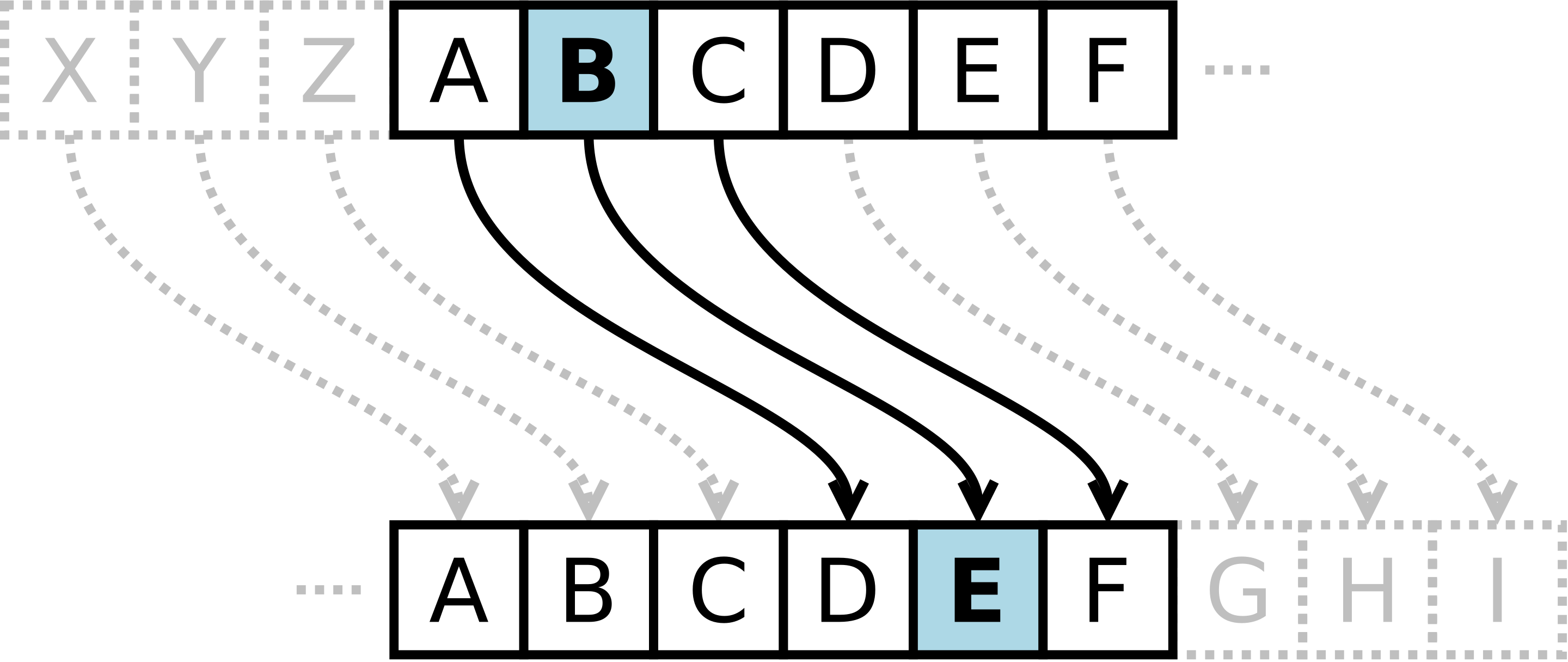

Cryptography, Cryptanalysis, Cryptology​

• Cryptography is the process of creating algorithms and protocols that are used for security purposes. It is often used interchangeably with cryptology.
• Cryptanalysis is the process of breaking cryptography.
• Cryptology refers to both cryptography and cryptanalysis, but this term is becoming less common.

Shift Cipher(Caesar’s cipher)​

• Each letter in the plaintext is replaced by a letter K positions ahead of it in the alphabet.
• An attacker can find K by trying every possible key since there are only 25 possible keys or fewer(key 0 return plaintext).
• Once K is found, encryption is very easy.

Substitution Cipher​

• Each letter X in the plaintext P is replaced with Y.
• They dominated the art of secret writing throughout the first millennium A.D.
• They were thought to be unbreakable by many back then.
• Substitution ciphers are vulnerable to frequency analysis attacks. Each language has certain features such as the frequency of letters or groups of two or more letters.

One-Time Pad (OTP)​

• OTP improves substitution cipher by using different keys to encrypt letters in different positions.
• The key should be a random string that is at least as long as the plaintext, according to Shannon's theorem.
• Shannon's theory states that the ciphertext should not reveal any information about the plaintext.
• Encryption is similar to the shift cipher.
• OTP was invented by Vernam in the 1920s.
• Never use the same key in OTP more than once.

Stream Cipher​

• The One-Time Pad encryption method uses a random key that is at least as long as the message being encrypted.
• Stream ciphers use a Pseudo Random Number Generator (PRNG) to create a sequence of numbers that appear random.
• Stream ciphers are usually fast.
• RC4 is a proprietary stream cipher owned by RSA, which became public in 1994.
• SSL/TLS uses RC4. SSLv3 does not have any major known vulnerabilities.
• If the same stream is used more than once, it becomes easy to break.
• These vulnerabilities are basic and still exist regardless of the strength of the PRNG.

Pseudo Random Number Generator (PRNG)​

• A PRNG is a tool used for cryptography and simulation.
• When using the same seed, a PRNG will always give the same output stream.
• For a PRNG to be cryptographically secure, it needs to have unpredictable sequences.
• PRNGs are also useful for generating temporary keys and other similar tasks.

Adversarial Models for Ciphers​

• The attacker is supposed to know the language of the original message and the type of encryption used.
• Ciphertext-only attack: The attacker can only see some encrypted messages.
• Known-plaintext attack: The attacker has seen some pairs of encrypted and decrypted messages.
• Chosen-plaintext attack: The attacker can choose some messages and see the corresponding encrypted messages.
• Chosen-ciphertext attack: The attacker can choose some encrypted messages and see the corresponding decrypted messages.

Data Encryption Standard (DES)​

• DES was designed by IBM with modifications proposed by the National Security Agency.
• From 1977 to 2001, it was a US national standard.
• It uses a block size of 64 bits and a key size of 56 bits.
• It has 16 rounds and was mostly designed for hardware implementations.
• However, it is now considered insecure and vulnerable to brute-force attacks.

Data Integrity and Source Authentication​

Encryption does not fully protect data from being changed by someone else. To make sure the data gets to its destination without being changed and to make sure it comes from a known source, we need something else.

Cryptographic Hash Function​

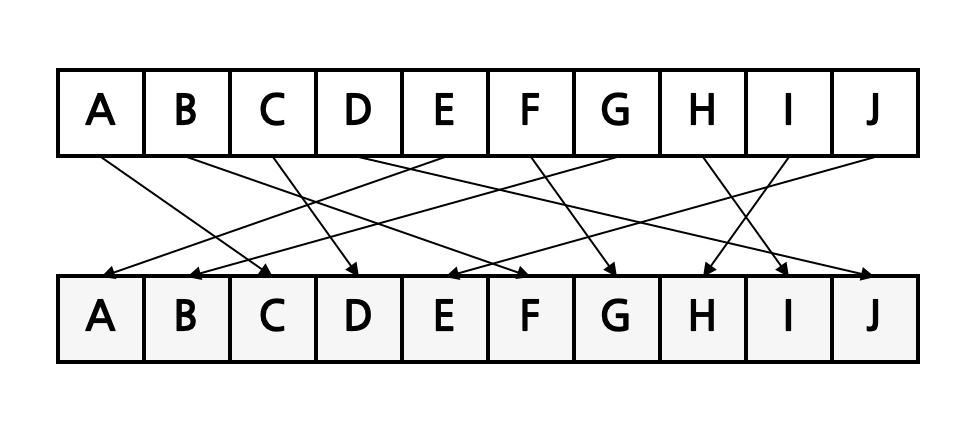
A hash function maps a message of arbitrary length to an m-bit output.

Since a hash function is a many-to-one function, collisions can occur.

Hash functions are used for the following examples:

• Software integrity
• Timestamping
• Message authentication
• One-time passwords
• Digital signatures

Well-known hash functions​

• MD5 - produces a 128-bit output. It has been completely broken by researchers in terms of collision resistance.
• SHA1 - produces a 160-bit output. No collisions have been found yet, but there is a method to find collisions in less than 2^80 attempts. It is considered insecure for collision resistance.
• SHA2 (SHA-224, SHA-256, SHA-384, SHA-512) - produces 224, 256, 384, and 512 bits output, respectively.
• Hash outputs should generally be twice the key length of block ciphers due to the birthday attack.

Limitations of Using Hash Functions for Authentication:​

• Anyone can calculate the hash of a message, since the hash function is public.
• It is not always possible to have a secure channel.

To fix these issues, you can:

• Use multiple hash functions.
• Select a hash function with a key.

Encryption and Authentication (3 Ways)​

• Authenticate-then-encrypt (AtE): This method is used in SSL. However, AtE may not always be secure because the first step is decryption, which can reveal whether the decryption was successful or not.
• Encrypt-then-authenticate (EtA): This method is used in IPSec. Encryption alone may not be enough to ensure privacy. EtA is a secure option.
• Encrypt-and-authenticate (E&A): This method is used in SSH. However, the MAC method does not guarantee confidentiality.

RSA Algorithm​

The most common public-key algorithm is called the RSA method, named after its inventors (Rivest, Shamir, Adleman). In this algorithm, the private key is a pair of numbers (N, d), and the public key is a pair of numbers (N, e). It should be noted that N is common to both the private and public keys.

Given a weighted graph and two vertices u and v, find a path of minimum total weight between u and v

applications:

• internet packet routing
• flight reservations
• driving directions

single source on unweighted graph ⇒ just use BFS

Dijkstra algorithm​

This algorithm constructs the shortest path tree from a source node. It does not allow negative edge weights and is similar to Prim's algorithm. The algorithm employs a greedy strategy and has a complexity of O(|E| + |V|log|V|). It is widely used in various applications, such as artificial satellite GPS software. Since negative edges do not usually exist in the real world, Dijkstra's algorithm is one of the most suitable algorithms for practical use.

1. Set the starting node.
2. Save the minimum cost of each node based on the starting node.
3. Select the node with the lowest cost among the nodes that have not been visited.
4. Consider the case of going to a specific node through the selected node and update the minimum cost.
5. Repeat steps 3-4 until all nodes have been visited.

Bellman-ford algorithm​

When all edge costs are positive, you can use Dijkstra's algorithm. However, if there are negative edges and negative cycles, a node with negative infinity occurs. In this case, you should use the Bellman-Ford algorithm. The Bellman-Ford algorithm can be used in situations involving negative edges and can detect negative cycles. The basic time complexity of the Bellman-Ford algorithm is O(VE), slower than Dijkstra's algorithm.

1. Choose a starting node.
2. Initialize the shortest distance table as infinite.
3. Repeat the following process n-1 times: Check each of the total e edges one by one. Calculate the cost of going to other nodes through each edge and update the shortest distance table.
4. If you want to check for the existence of a negative cycle, repeat step 3. once more. If the shortest distance table is updated this time, a negative cycle exists.

Floyd-Warshall​

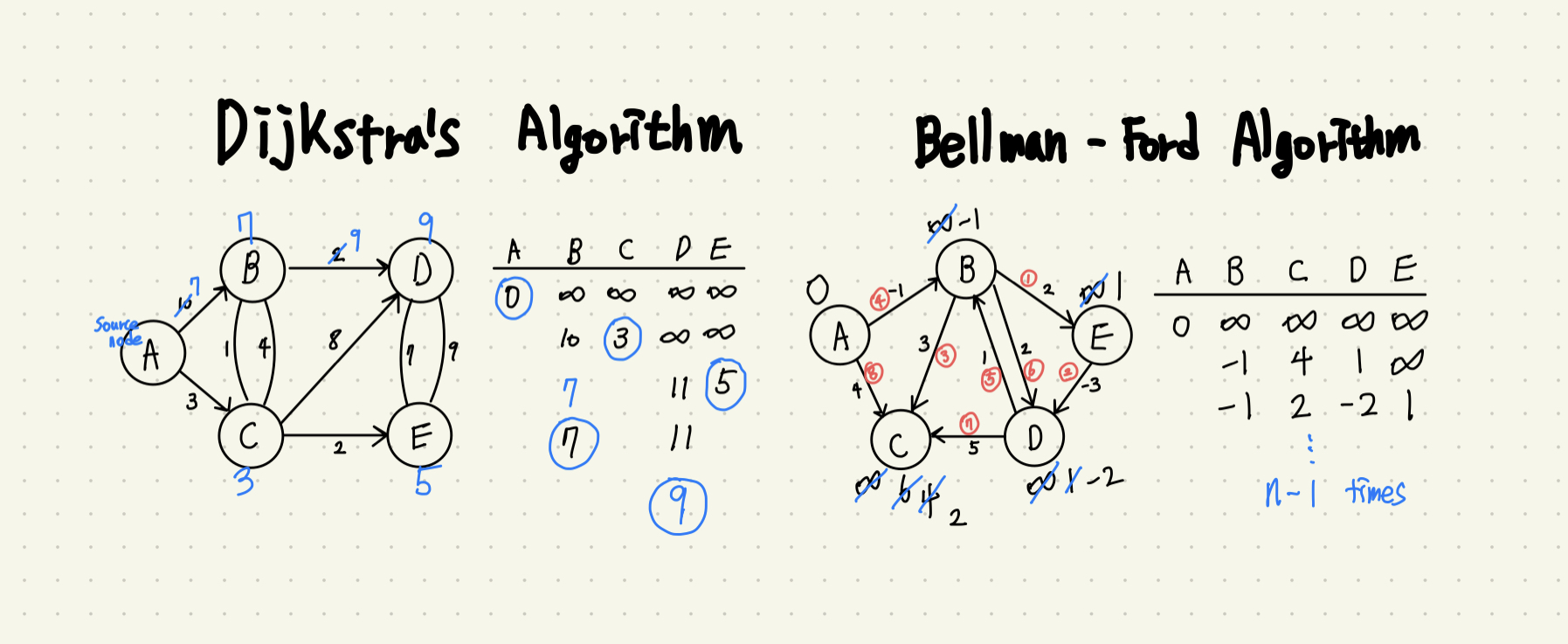
Dijkstra's and Bellman-Ford algorithms are algorithms that find the shortest path from one vertex to another when starting from a single vertex. However, if you want to find the shortest paths between all pairs of vertices, you need to use the Floyd-Warshall algorithm. While Dijkstra's algorithm chooses the least cost one by one, the Floyd-Warshall algorithm performs the algorithm based on the intermediate vertex.

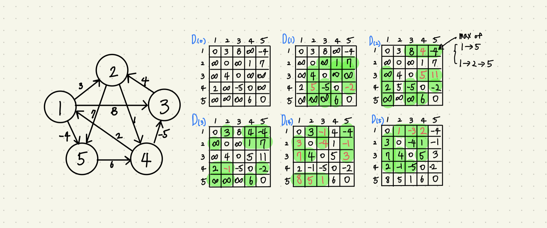
The green zone is a changeable area. Nodes with self-loops and containing intermediate vertices are not able to be changed.

The key idea of the Floyd-Warshall algorithm is to find the shortest distance based on the intermediate vertex. Calculate the number of cases where all n nodes are passed through.

The time complexity is O(V^3).